|
Tamaño: 2103
Comentario:
|
Tamaño: 3662
Comentario:
|
| Los textos eliminados se marcan así. | Los textos añadidos se marcan así. |
| Línea 42: | Línea 42: |
| * Classification results on the SFB (left) and FL (right) images: | ==== Mean accuracy on SFB and FL for the CWC, RWM and the FV-based approaches ==== <<BR>> || '''Dataset''' || '''CWC''' || '''RWM''' ($K$=32, $n$=3) || '''Ours''' ($K$=16, $n$=5)|| || '''SFB''' || 0.8848 (0.0602) || 0.9081 (0.0238) || 0.9707 (0.0079) || || '''FL''' || 0.8762 (0.0223) || 0.8608 (0.0312) || 0.9144 (0.0191) || <<BR>> ==== Classification results on the SFB (left) and FL (right) images ==== <<BR>> {{attachment:sfb_segmentation.png || width=200}} {{attachment:fl_segmentation.png || width=200}} <<BR>> ==== Comparison with the best performing method of [1] in FL ==== <<BR>> || '''Method''' || BareSoil || Beet || Forest || Grasses || Lucerne || Peas || Potatoes || Rapeseed || Beans || Water || Wheat || Mean || || Wang etal. [1] || 0.9878 || 0.9371 || 0.9496 || 0.8489 || 0.9231 || 0.9555 || 0.8896 || 0.9486 || 0.9653 || 0.9642 || 0.8864 || 0.9324 || || Ours ($K=16, n=5$) || 1.0 || 0.9926 || 0.9770 || 0.9920 || 0.9261 || 0.9993 || 0.9959 || 0.9983 || 0.9757 || 0.8472 || 0.9971 || 0.9728 || <<BR>> ==== Comparison with [2] in FL ==== <<BR>> || '''Method''' || Accuracy || || W-DSN [2] || 0.9268 (-) || || Ours ($K$=16, $n$=5) || 0.9688 (0.0062) || <<BR>> === References === |
| Línea 44: | Línea 66: |
| {{attachment:sfb_segmentation.png || width=200}} {{attachment:fl_segmentation.png || width=200}} | [1] H. Wang, Z. Zhou, J. Turnbull, Q. Song, and F. Qi, “Pol-SAR classification based on generalized polar decomposition of mueller matrix,” IEEE Geosc. Remote Sens. Lett., vol. 13, no. 4, pp. 565–569, 2016. [2] L. Jiao and F. Liu, “Wishart deep stacking network for fast polsar image classification,” IEEE Trans. Image Process., vol. 25, no. 7, pp. 3273–3286, 2016. |
Fisher Vectors for PolSAR Image Classification
Abstract
In this letter we study the application of the Fisher Vector (FV) to the problem of pixel-wise supervised classification of PolSAR images. This is a challenging problem since information in those images is encoded as complex-valued covariance matrices. We observe that the real part of these matrices preserve the positive semidefiniteness property of their complex counterpart. Based on this observation, we derive a FV from a mixture of real Wishart pdfs and integrate it with a Potts-like energy model in order to capture spatial dependencies between neighboring regions. Experimental results on two challenging datasets show the effectiveness of the approach.
Paper
Javier Redolfi, Jorge Sánchez, and Ana Georgina Flesia
"Fisher Vectors for PolSAR Image Classification"
IEEE Geoscience and Remote Sensing Letters (Accepted with Major Changes)
Code
Dataset
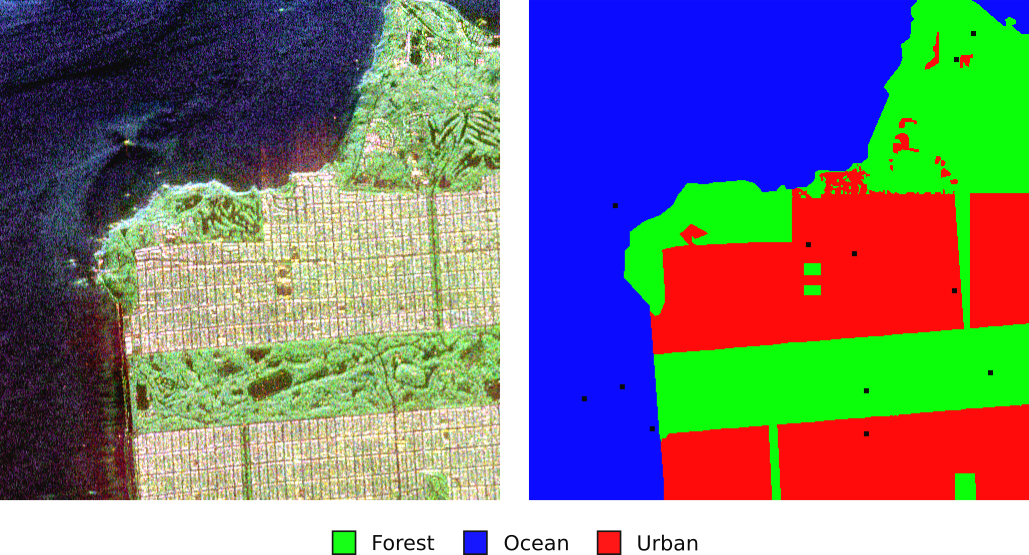
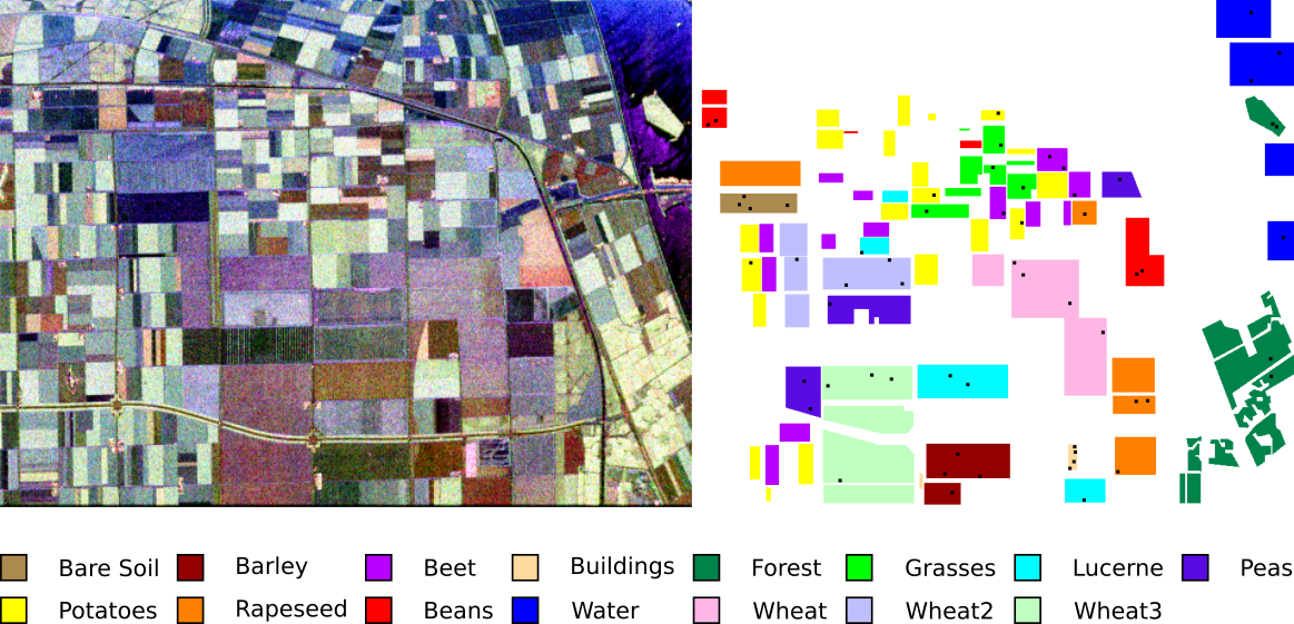
For evaluation, we consider a subset of the images that were available trough PolSARpro by the European Space Agency (ESA). This subset consists of two fully polarimetric images over the San Francisco Bay (SFB) area, USA, and over an agricultural region in the Flevoland (FL) province in The Netherlands.
The dataset and a set of ground truth annotations will be available upon approval of the manupscript.
San Francisco Bay
Pseudocolor representation of the polarimetric data (left) and the ground truth labels (right).

Flevoland
Pseudocolor representation of the polarimetric data (left) and the ground truth labels (right).

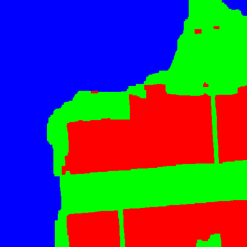
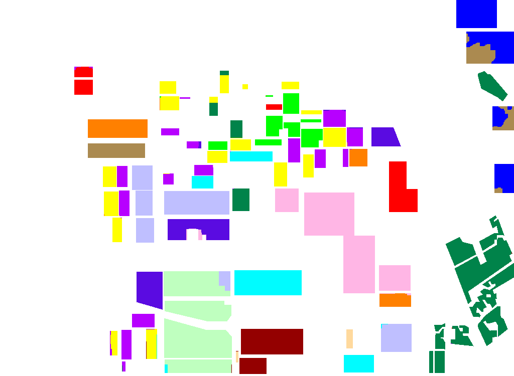
Classification Examples
Mean accuracy on SFB and FL for the CWC, RWM and the FV-based approaches
Dataset |
CWC |
RWM ($K$=32, $n$=3) |
Ours ($K$=16, $n$=5) |
SFB |
0.8848 (0.0602) |
0.9081 (0.0238) |
0.9707 (0.0079) |
FL |
0.8762 (0.0223) |
0.8608 (0.0312) |
0.9144 (0.0191) |
Classification results on the SFB (left) and FL (right) images


Comparison with the best performing method of [1] in FL
Method |
Beet |
Forest |
Grasses |
Lucerne |
Peas |
Potatoes |
Rapeseed |
Beans |
Water |
Wheat |
Mean |
|
Wang etal. [1] |
0.9878 |
0.9371 |
0.9496 |
0.8489 |
0.9231 |
0.9555 |
0.8896 |
0.9486 |
0.9653 |
0.9642 |
0.8864 |
0.9324 |
Ours ($K=16, n=5$) |
1.0 |
0.9926 |
0.9770 |
0.9920 |
0.9261 |
0.9993 |
0.9959 |
0.9983 |
0.9757 |
0.8472 |
0.9971 |
0.9728 |
Comparison with [2] in FL
Method |
Accuracy |
W-DSN [2] |
0.9268 (-) |
Ours ($K$=16, $n$=5) |
0.9688 (0.0062) |
References
[1] H. Wang, Z. Zhou, J. Turnbull, Q. Song, and F. Qi, “Pol-SAR classification based on generalized polar decomposition of mueller matrix,” IEEE Geosc. Remote Sens. Lett., vol. 13, no. 4, pp. 565–569, 2016.
[2] L. Jiao and F. Liu, “Wishart deep stacking network for fast polsar image classification,” IEEE Trans. Image Process., vol. 25, no. 7, pp. 3273–3286, 2016.

